Least Squares
안녕하세요. 오태호입니다.
이 글에서는 Least Squares와 관련된 몇 가지 수식을 유도하여 Least Squares에 대해 이해를 해 보도록 하겠습니다.
이 글을 이해하기 위해서는 Linear Algebra, Statistics에 대한 기초지식이 필요합니다.
Matrix나 Vector는 굵은 글꼴로 표현하도록 하겠습니다. 그리고 Vector는 특별히 언급이 없으면 Column Vector를 의미합니다.
Projection
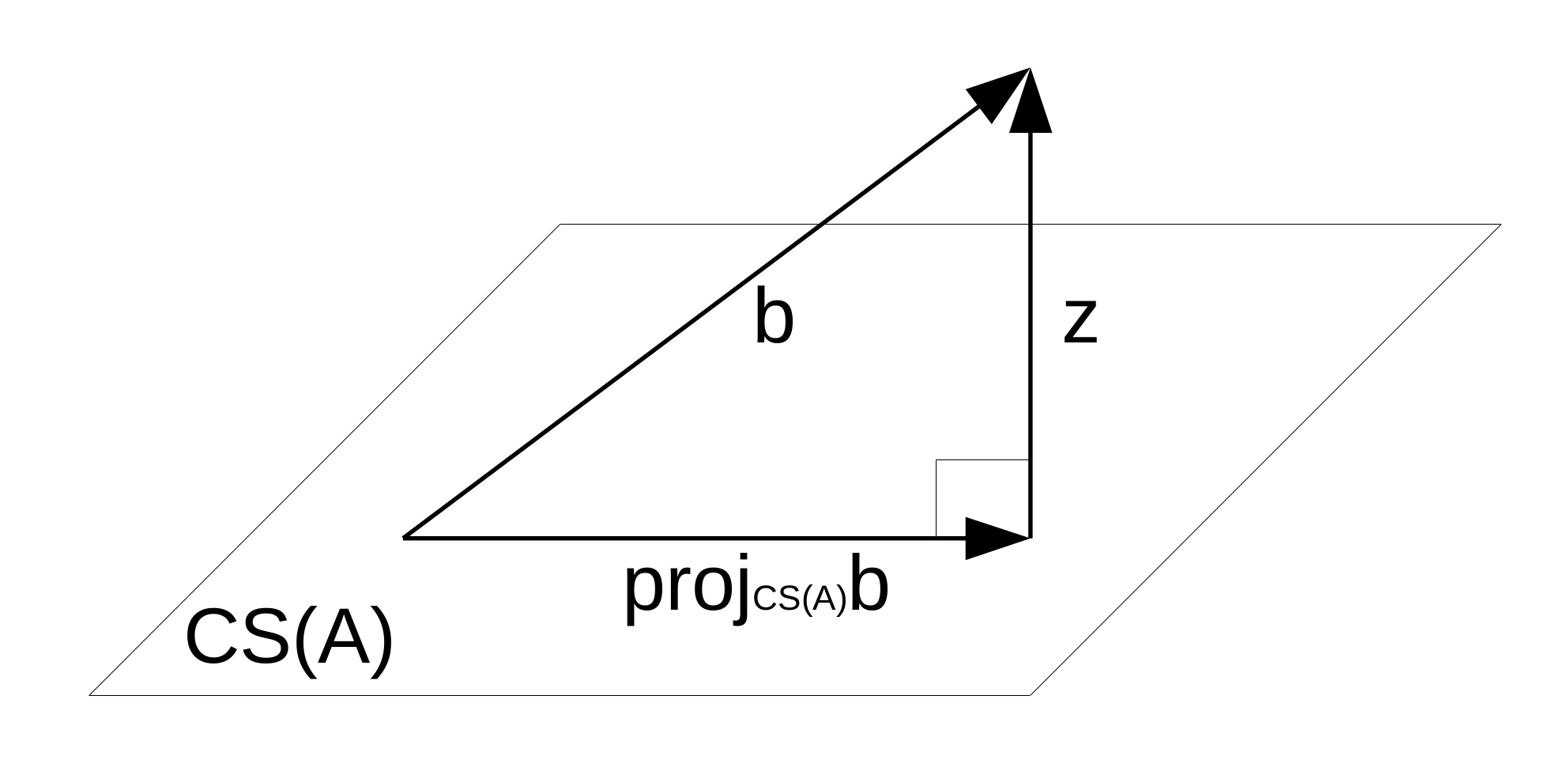
\(\mathbf A\)는 \(m \times n\)의 Matrix이고, \(\mathbf{b}\)는 \(m \times 1\)의 Vector일 때, \(\mathbf{b}\)의 \(\mathbf A\)의 Column Space \(CS(\mathbf{A})\)에 대한 Projection Vector \(proj_{CS(\mathbf A)}\mathbf{b}\)는 다음과 같이 계산합니다.
\(\mathbf{x}\)는 \(n \times 1\)의 Vector이고 다음과 같이 정의합니다.
\[proj_{CS(\mathbf A)}\mathbf{b}=\mathbf{A}\mathbf{x}\]\(proj_{CS(\mathbf A)}\mathbf{b}\)는 \(\mathbf{A}\)의 Column Vector들을 Linear Combination한 Vector이므로 \(\mathbf{A}\mathbf{x}\)와 같이 표현이 가능합니다.
\(\mathbf{z}\)는 \(m \times 1\)의 Vector이고 다음과 같이 정의합니다.
\[\mathbf{z}=\mathbf{b}-proj_{CS(\mathbf A)}\mathbf{b}\]아래 그림을 살펴보면 \(\mathbf{z}\)는 \(CS(\mathbf{A})\)의 Orthogonal Complement에 속해 있는 Vector라는 사실을 알 수 있습니다.
\(CS(\mathbf{A})^\perp\)는 \(\mathbf{A}\)의 Column Space의 Orthogonal Complement를 의미합니다. 즉, \(\mathbf{A}\)의 모든 Column Vector들과 Orthogonal한 Vector들로 이루어진 Vector Space를 의미합니다. 다시 말하면, \(\mathbf{A}\)의 모든 Column Vector들과 Dot Product가 \(0\)이 되는 Vector들로 이루어진 Vector Space를 의미합니다.
\(Null(\mathbf{A}^T)\)는 \(\mathbf{A}^T\mathbf{h}=\mathbf{0}\)을 만족하는 \(\mathbf{h}\)들로 이루어진 Vector Space를 의미합니다. 즉, \(\mathbf{A}^T\)의 모든 Row Vector들과 Dot Product가 \(0\)가 되는 Vector들로 이루어진 Vector Space를 의미하고, 이것은 \(\mathbf{A}\)의 모든 Column Vector들과 Dot Product가 \(0\)이 되는 Vector들로 이루어진 Vector Space를 의미하며, 결국에 \(CS(\mathbf{A})^\perp\)과 동일한 Vector Space를 의미합니다.
\[\mathbf{A}^T\mathbf{z}=\mathbf{0} \\ \mathbf{A}^T(\mathbf{b}-proj_{CS(\mathbf A)}\mathbf{b})=\mathbf{0} \\ \mathbf{A}^T(\mathbf{b}-\mathbf{A}\mathbf{x})=\mathbf{0} \\ \mathbf{A}^T\mathbf{b}-\mathbf{A}^T\mathbf{A}\mathbf{x}=\mathbf{0} \\ \mathbf{x}=(\mathbf{A}^T\mathbf{A})^{-1}\mathbf{A}^T\mathbf{b} \\ \begin{aligned} proj_{CS(\mathbf A)}\mathbf{b} &=\mathbf{A}\mathbf{x} \\ &=\mathbf{A}(\mathbf{A}^T\mathbf{A})^{-1}\mathbf{A}^T\mathbf{b} \end{aligned}\]정리하면 다음과 같습니다.
\[proj_{CS(\mathbf A)}\mathbf{b}=\mathbf{A}(\mathbf{A}^T\mathbf{A})^{-1}\mathbf{A}^T\mathbf{b}\]Ordinary Least Squares
\(\mathbf A\)는 \(m \times n\)의 Matrix, \(\mathbf{x}\)는 \(n \times 1\)의 Vector, \(\mathbf{b}\)는 \(m \times 1\)의 Vector라고 정의합니다. \(\mathbf A\)와 \(\mathbf b\)의 값이 주어졌을 때 \(\min_\mathbf{x} \left \| \mathbf{A}\mathbf{x}-\mathbf{b} \right \|_2^2\)을 만족하는 \(\mathbf x\)는 다음과 같이 계산합니다.
\(\mathbf{A}\mathbf{x}\)에서 \(\mathbf{x}\)는 임의의 값을 가질 수 있는 Vector이고, \(\mathbf{A}\mathbf{x}\)는 \(\mathbf{A}\)의 Column Space상의 임의의 Vector를 표현할 수 있습니다. \(\mathbf{b}\)와 \(\mathbf{A}\mathbf{x}\)의 거리가 가장 가까운 지점은, \(\mathbf{b}\)와 \(\mathbf{A}\)의 Column Space상에서 가장 거리가 가까운 지점이 됩니다. 이 지점은 \(\mathbf{b}\)에서 \(\mathbf{A}\)의 Column Space에 수직이 되는 지점으로, 즉, \(\mathbf{b}\)를 \(\mathbf{A}\)의 Column Space에 Projection한 지점입니다. 이것을 정리해서 표현하면 \(proj_{CS(\mathbf A)}\mathbf{b}\)이 됩니다. 이 사실을 바탕으로 \(\mathbf{A}\mathbf{x}\)를 구하고 \(\mathbf{x}\)를 구합니다.
\[\begin{aligned} \mathbf{A}\mathbf{x} &=proj_{CS(\mathbf A)}\mathbf{b} \\ &=\mathbf{A}(\mathbf{A}^T\mathbf{A})^{-1}\mathbf{A}^T\mathbf{b} \\ \end{aligned} \\ \mathbf{x}=(\mathbf{A}^T\mathbf{A})^{-1}\mathbf{A}^T\mathbf{b}\]정리하면 다음과 같습니다.
\[\underset{\mathbf{x}}{\mathrm{argmin}} \left \| \mathbf{A}\mathbf{x}-\mathbf{b} \right \|_2^2 = (\mathbf{A}^T\mathbf{A})^{-1}\mathbf{A}^T\mathbf{b}\]Regularized Least Squares
\(\mathbf A\)는 \(m \times n\)의 Matrix, \(\mathbf{x}\)는 \(n \times 1\)의 Vector, \(\mathbf{b}\)는 \(m \times 1\)의 Vector라고 정의합니다. \(\mathbf A\)와 \(\mathbf b\)와 \(\lambda\)의 값이 주어졌을 때 \(\min_\mathbf{x} (\left \| \mathbf{A}\mathbf{x}-\mathbf{b} \right \|_2^2 + \lambda \left \| \mathbf{x} \right \|_2^2)\)을 만족하는 \(\mathbf x\)는 다음과 같이 계산합니다.
직관적으로는 다음과 같이 이해할 수 있습니다.
\(\mathbf{A}\)는 Model 학습을 위한 Input Data이고 \(\mathbf{b}\)는 Model 학습을 위한 Output Data입니다. Input Data가 주어졌을 때 Output Data를 Prediction하는 Model을 만들고 싶습니다. Model의 Parameter는 \(\mathbf{x}\)입니다. \(\mathbf{A}\)의 각 Column은 각각이 Feature입니다. 특정 Feature에 지나치게 의존하게 되면 Overfit이 발생할 우려가 있으니 \(\mathbf{x}\) Vector의 특정 Element가 지나치게 커지는 것을 방지합니다. 그러기 위해서 \(\lambda \left \| \mathbf{x} \right \|_2^2\)이 지나치게 커지는 것을 방지하여 여러 Feature를 골고루 바라보도록 유도합니다. 극단적으로 \(\lambda\)가 \(\infty\)의 값을 가지면 \(\mathbf{x}\)가 \(\mathbf{0}\)이 되면서 Underfit이 발생하고 \(\lambda\)가 \(0\)의 값을 가지면 Ordinary Least Squares와 동일한 형태가 되면서 Overfit이 발생할 위험이 있습니다.
\[\min_\mathbf{x} (\left \| \mathbf{A}\mathbf{x}-\mathbf{b} \right \|_2^2 + \lambda \left \| \mathbf{x} \right \|_2^2) =\min_\mathbf{x} \left \| \begin{bmatrix} \mathbf{A} \\ \sqrt{\lambda}\mathbf{I} \end{bmatrix} \mathbf{x} - \begin{bmatrix} \mathbf{b} \\ \mathbf{0} \end{bmatrix} \right \|_2^2 \\ \begin{aligned} \underset{\mathbf{x}}{\mathrm{argmin}} \left \| \begin{bmatrix} \mathbf{A} \\ \sqrt{\lambda}\mathbf{I} \end{bmatrix} \mathbf{x} - \begin{bmatrix} \mathbf{b} \\ \mathbf{0} \end{bmatrix} \right \|_2^2 &= \left ( \begin{bmatrix} \mathbf{A} \\ \sqrt{\lambda}\mathbf{I} \end{bmatrix}^T \begin{bmatrix} \mathbf{A} \\ \sqrt{\lambda}\mathbf{I} \end{bmatrix} \right )^{-1} \begin{bmatrix} \mathbf{A} \\ \sqrt{\lambda}\mathbf{I} \end{bmatrix}^T \begin{bmatrix} \mathbf{b} \\ \mathbf{0} \end{bmatrix} \\ &= \left ( \begin{bmatrix} \mathbf{A}^T & \sqrt{\lambda}\mathbf{I} \end{bmatrix} \begin{bmatrix} \mathbf{A} \\ \sqrt{\lambda}\mathbf{I} \end{bmatrix} \right )^{-1} \begin{bmatrix} \mathbf{A}^T & \sqrt{\lambda}\mathbf{I} \end{bmatrix} \begin{bmatrix} \mathbf{b} \\ \mathbf{0} \end{bmatrix} \\ &= (\mathbf{A}^T\mathbf{A}+\lambda\mathbf{I})^{-1}\mathbf{A}^T\mathbf{b} \end{aligned}\]정리하면 다음과 같습니다.
\[\underset{\mathbf{x}}{\mathrm{argmin}}(\left \| \mathbf{A}\mathbf{x}-\mathbf{b} \right \|_2^2 + \lambda \left \| \mathbf{x} \right \|_2^2)=(\mathbf{A}^T\mathbf{A}+\lambda\mathbf{I})^{-1}\mathbf{A}^T\mathbf{b}\]정확한 정의는 조금씩 차이가 있지만 이 방법은 L2 Regularization, Tikhonov Regularization, Ridge Regression라고도 불립니다.
Multi Objective Least Squares
\(\mathbf{A}_i\)는 \(m \times n\)의 Matrix, \(\mathbf{x}\)는 \(n \times 1\)의 Vector, \(\mathbf{b}_i\)는 \(m \times 1\)의 Vector라고 정의합니다. \(\mathbf{A}_i\)와 \(\mathbf{b}_i\)와 \(\lambda_i\)의 값이 주어졌을 때 \(\min_\mathbf{x} \left (\sum_{i=1}^k \lambda_i \left \| \mathbf{A}_i\mathbf{x}-\mathbf{b}_i \right \|_2^2 \right )\)을 만족하는 \(\mathbf x\)는 다음과 같이 계산합니다.
직관적으로는 다음과 같이 이해할 수 있습니다.
\(\mathbf{A}_i\)는 Model 학습을 위한 Input Data이고 \(\mathbf{b}_i\)는 Model 학습을 위한 Output Data입니다. Input Data가 주어졌을 때 Output Data를 Prediction하는 Model을 만들고 싶습니다. Model의 Parameter는 \(\mathbf{x}\)입니다. Input Data와 Output Data를 여러 Group으로 나누고 Group마다 \(\lambda_i\)로 가중치를 줘서 특정 Group의 Data를 더 중요하게 생각해서 Model을 만듭니다. 특정 Group의 \(\mathbf{A}_i\)를 \(\mathbf{I}\)로 설정하고 \(\mathbf{b}_i\)를 \(\mathbf{0}\)으로 설정하고 \(\lambda_i\)를 적절하게 설정해 주면 Regularized Least Squares와 동일한 형태가 됩니다.
\[\min_\mathbf{x} \left (\sum_{i=1}^k \lambda_i \left \| \mathbf{A}_i\mathbf{x}-\mathbf{b}_i \right \|_2^2 \right ) =\min_\mathbf{x} \left \| \begin{bmatrix} \sqrt{\lambda_1}\mathbf{A}_1 \\ \sqrt{\lambda_2}\mathbf{A}_2 \\ \vdots \\ \sqrt{\lambda_k}\mathbf{A}_k \\ \end{bmatrix} \mathbf{x} - \begin{bmatrix} \sqrt{\lambda_1}\mathbf{b}_1 \\ \sqrt{\lambda_2}\mathbf{b}_2 \\ \vdots \\ \sqrt{\lambda_k}\mathbf{b}_k \\ \end{bmatrix} \right \|_2^2 \\ \begin{aligned} \underset{\mathbf{x}}{\mathrm{argmin}}\left \| \begin{bmatrix} \sqrt{\lambda_1}\mathbf{A}_1 \\ \sqrt{\lambda_2}\mathbf{A}_2 \\ \vdots \\ \sqrt{\lambda_k}\mathbf{A}_k \\ \end{bmatrix} \mathbf{x} - \begin{bmatrix} \sqrt{\lambda_1}\mathbf{b}_1 \\ \sqrt{\lambda_2}\mathbf{b}_2 \\ \vdots \\ \sqrt{\lambda_k}\mathbf{b}_k \\ \end{bmatrix} \right \|_2^2 &= \left ( \begin{bmatrix} \sqrt{\lambda_1}\mathbf{A}_1 \\ \sqrt{\lambda_2}\mathbf{A}_2 \\ \vdots \\ \sqrt{\lambda_k}\mathbf{A}_k \end{bmatrix}^T \begin{bmatrix} \sqrt{\lambda_1}\mathbf{A}_1 \\ \sqrt{\lambda_2}\mathbf{A}_2 \\ \vdots \\ \sqrt{\lambda_k}\mathbf{A}_k \end{bmatrix} \right )^{-1} \begin{bmatrix} \sqrt{\lambda_1}\mathbf{A}_1 \\ \sqrt{\lambda_2}\mathbf{A}_2 \\ \vdots \\ \sqrt{\lambda_k}\mathbf{A}_k \end{bmatrix}^T \begin{bmatrix} \sqrt{\lambda_1}\mathbf{b}_1 \\ \sqrt{\lambda_2}\mathbf{b}_2 \\ \vdots \\ \sqrt{\lambda_k}\mathbf{b}_k \\ \end{bmatrix} \\ &= \left (\sum_{i=1}^k\lambda_i\mathbf{A}_i^T\mathbf{A}_i \right )^{-1} \left (\sum_{i=1}^k\lambda_i\mathbf{A}_i^T\mathbf{b}_i \right ) \end{aligned}\]정리하면 다음과 같습니다.
\[\underset{\mathbf{x}}{\mathrm{argmin}}\left (\sum_{i=1}^k \lambda_i \left \| \mathbf{A}_i\mathbf{x}-\mathbf{b}_i \right \|_2^2 \right )=\left (\sum_{i=1}^k\lambda_i\mathbf{A}_i^T\mathbf{A}_i \right )^{-1} \left (\sum_{i=1}^k\lambda_i\mathbf{A}_i^T\mathbf{b}_i \right )\]Weighted Least Squares
\(\mathbf A\)는 \(m \times n\)의 Matrix, \(\mathbf{x}\)는 \(n \times 1\)의 Vector, \(\mathbf{b}\)는 \(m \times 1\)의 Vector, \(\mathbf{W}\)는 \(m \times m\)의 Diagonal Matrix라고 정의합니다. \(\mathbf A\)와 \(\mathbf b\)와 \(\mathbf{W}\)의 값이 주어졌을 때 \(\min_\mathbf{x} (\mathbf{A}\mathbf{x}-\mathbf{b})^T\mathbf{W}(\mathbf{A}\mathbf{x}-\mathbf{b})\)을 만족하는 \(\mathbf x\)는 다음과 같이 계산합니다.
\(\mathbf{W}\)와 \(\sqrt{\mathbf{W}}\)는 다음과 같이 정의합니다.
\[\mathbf{W}= \begin{bmatrix} w_1 && 0 && \cdots && 0 \\ 0 && w_2 && \cdots && 0 \\ \vdots && \vdots && \ddots && \vdots \\ 0 && 0 && \cdots && w_m \end{bmatrix} \\ \sqrt{\mathbf{W}}= \begin{bmatrix} \sqrt{w_1} && 0 && \cdots && 0 \\ 0 && \sqrt{w_2} && \cdots && 0 \\ \vdots && \vdots && \ddots && \vdots \\ 0 && 0 && \cdots && \sqrt{w_m} \end{bmatrix}\]직관적으로는 다음과 같이 이해할 수 있습니다.
\(\mathbf{A}\)는 Model 학습을 위한 Input Data이고 \(\mathbf{b}\)는 Model 학습을 위한 Output Data입니다. Input Data가 주어졌을 때 Output Data를 Prediction하는 Model을 만들고 싶습니다. Model의 Parameter는 \(\mathbf{x}\)입니다. \(\mathbf{A}\)의 각 Row는 각각이 Data Point입니다. Model의 경우에는 Input으로 동일한 Data Point가 주어지면 Model의 Output이 동일하지만, 실제 수집된 Output Data \(\mathbf{b}\)의 Data Point는 여러가지 이유로(측정오류 등) 값이 흔들리게 됩니다. 어떤 Input Data의 Data Point의 경우에는 Output이 크게 흔들리고 어떤 Input Data의 Data Point의 경우에는 Output이 작게 흔들릴 수 있습니다. 이런 상황을 Heteroskedasticity가 존재한다고 말합니다. 이런 경우에 그대로 Model을 학습하게 되면 Output이 크게 흔들리는 경우를 좀 더 중요하게 생각해서 학습이 이루어지게 됩니다. 그래서 이런 상황에는 Output이 크게 흔들리는 경우에는 Weight를 작게 주고 Output이 작게 흔들리는 경우에는 Weight를 크게 줘서 Model을 균형있게 학습시킵니다. Weight는 \(\mathbf{W}\)에 설정합니다.
\[\begin{aligned} \min_\mathbf{x} (\mathbf{A}\mathbf{x}-\mathbf{b})^T\mathbf{W}(\mathbf{A}\mathbf{x}-\mathbf{b}) &=\min_\mathbf{x} (\mathbf{A}\mathbf{x}-\mathbf{b})^T(\sqrt{\mathbf{W}})^T(\sqrt{\mathbf{W}})(\mathbf{A}\mathbf{x}-\mathbf{b}) \\ &=\min_\mathbf{x} (\sqrt{\mathbf{W}}\mathbf{A}\mathbf{x}-\sqrt{\mathbf{W}}\mathbf{b})^T(\sqrt{\mathbf{W}}\mathbf{A}\mathbf{x}-\sqrt{\mathbf{W}}\mathbf{b}) \\ &=\min_\mathbf{x} \left \| \sqrt{\mathbf{W}}\mathbf{A}\mathbf{x}-\sqrt{\mathbf{W}}\mathbf{b} \right \|_2^2 \end{aligned} \\ \begin{aligned} \underset{\mathbf{x}}{\mathrm{argmin}}\left \| \sqrt{\mathbf{W}}\mathbf{A}\mathbf{x}-\sqrt{\mathbf{W}}\mathbf{b} \right \|_2^2 &=((\sqrt{\mathbf{W}}\mathbf{A})^T(\sqrt{\mathbf{W}}\mathbf{A}))^{-1}(\sqrt{\mathbf{W}}\mathbf{A})^T(\sqrt{\mathbf{W}}\mathbf{b}) \\ &=(\mathbf{A}^T\mathbf{W}\mathbf{A})^{-1}\mathbf{A}^T\mathbf{W}\mathbf{b} \end{aligned}\]정리하면 다음과 같습니다.
\[\underset{\mathbf{x}}{\mathrm{argmin}}(\mathbf{A}\mathbf{x}-\mathbf{b})^T\mathbf{W}(\mathbf{A}\mathbf{x}-\mathbf{b})=(\mathbf{A}^T\mathbf{W}\mathbf{A})^{-1}\mathbf{A}^T\mathbf{W}\mathbf{b}\]Generalized Least Squares
\(\mathbf A\)는 \(m \times n\)의 Matrix, \(\mathbf{x}\)는 \(n \times 1\)의 Vector, \(\mathbf{b}\)는 \(m \times 1\)의 Vector, \(\mathbf{C}\)는 \(m \times m\)의 Positive Definite Matrix라고 정의합니다. \(\mathbf A\)와 \(\mathbf b\)와 \(\mathbf{C}\)의 값이 주어졌을 때 \(\min_\mathbf{x} (\mathbf{A}\mathbf{x}-\mathbf{b})^T\mathbf{C}^{-1}(\mathbf{A}\mathbf{x}-\mathbf{b})\)을 만족하는 \(\mathbf x\)는 다음과 같이 계산합니다.
\(\mathbf{C}\)는 Positive Definite Matrix이므로 Cholesky Decomposition을 이용하여 아래와 같이 Decomposition할 수 있습니다.
\[\mathbf{C}=\mathbf{L}\mathbf{L}^T\]직관적으로는 다음과 같이 이해할 수 있습니다.
\(\mathbf{A}\)는 Model 학습을 위한 Input Data이고 \(\mathbf{b}\)는 Model 학습을 위한 Output Data입니다. Input Data가 주어졌을 때 Output Data를 Prediction하는 Model을 만들고 싶습니다. Model의 Parameter는 \(\mathbf{x}\)입니다. \(\mathbf{A}\)의 각 Row는 각각이 Data Point입니다. 첫 번째 Data Point에 대한 Output과 Model의 Output과 차이하고, 두 번째 Data Point에 대한 Output과 Model의 Output이 서로 Correlation이 있을 수 있습니다. 예를 들어, 첫 번째 Data Point에 대한 Output은 서울의 2021년 1월 1일의 온도이고 두 번째 Data Point에 대한 Output은 서울의 2021년 1월 2일의 온도라면, 첫 번째 Data Point의 Output과 Model의 Output과 차이하고, 두 번째 Data Point의 Output과 Model의 Output과 차이하고는, 서로 Correlation이 되어 있을 가능성이 높다는 것을 예상할 수 있습니다. 이런 경우에 \(\mathbf{L}^{-1}\) Matrix를 \(\mathbf{A}\)와 \(\mathbf{b}\)에 곱해서 Correlation이 제거된 Vector Space로 Transform한 후 Model을 학습시킵니다. \(\mathbf{C}\)는 Matrix는 Data Point의 Output과 Model의 Output과의 차이 값들의 Covariance Matrix로 설정합니다. 참고로 \(\mathbf{C}\) Matrix를 구하는 것이 현실적으로 힘든 경우가 많이 있는데 이런 경우에는 Generalized Least Squares을 사용하기가 어렵습니다. \(\mathbf{C}\) Matrix가 Diagonal Matrix라면 Correlation이 존재하지 않는 것을 의미하며 Weighted Least Squares와 동일한 형태가 됩니다.
\[\begin{aligned} \min_\mathbf{x} (\mathbf{A}\mathbf{x}-\mathbf{b})^T\mathbf{C}^{-1}(\mathbf{A}\mathbf{x}-\mathbf{b}) &=\min_\mathbf{x} (\mathbf{A}\mathbf{x}-\mathbf{b})^T(\mathbf{L}\mathbf{L}^T)^{-1}(\mathbf{A}\mathbf{x}-\mathbf{b}) \\ &=\min_\mathbf{x} (\mathbf{A}\mathbf{x}-\mathbf{b})^T(\mathbf{L}^{-1})^T(\mathbf{L}^{-1})(\mathbf{A}\mathbf{x}-\mathbf{b}) \\ &=\min_\mathbf{x} (\mathbf{L}^{-1}\mathbf{A}\mathbf{x}-\mathbf{L}^{-1}\mathbf{b})^T(\mathbf{L}^{-1}\mathbf{A}\mathbf{x}-\mathbf{L}^{-1}\mathbf{b}) \\ &=\min_\mathbf{x} \left \| \mathbf{L}^{-1}\mathbf{A}\mathbf{x}-\mathbf{L}^{-1}\mathbf{b} \right \|_2^2 \end{aligned} \\ \begin{aligned} \underset{\mathbf{x}}{\mathrm{argmin}}\left \| \mathbf{L}^{-1}\mathbf{A}\mathbf{x}-\mathbf{L}^{-1}\mathbf{b} \right \|_2^2 &=((\mathbf{L}^{-1}\mathbf{A})^T(\mathbf{L}^{-1}\mathbf{A}))^{-1}(\mathbf{L}^{-1}\mathbf{A})^T(\mathbf{L}^{-1}\mathbf{b}) \\ &=(\mathbf{A}^T(\mathbf{L}\mathbf{L}^T)^{-1}\mathbf{A})^{-1}\mathbf{A}^T(\mathbf{L}\mathbf{L}^T)^{-1}\mathbf{b} \\ &=(\mathbf{A}^T\mathbf{C}^{-1}\mathbf{A})^{-1}\mathbf{A}^T\mathbf{C}^{-1}\mathbf{b} \end{aligned}\]정리하면 다음과 같습니다.
\[\underset{\mathbf{x}}{\mathrm{argmin}}(\mathbf{A}\mathbf{x}-\mathbf{b})^T\mathbf{C}^{-1}(\mathbf{A}\mathbf{x}-\mathbf{b}) =(\mathbf{A}^T\mathbf{C}^{-1}\mathbf{A})^{-1}\mathbf{A}^T\mathbf{C}^{-1}\mathbf{b}\]\(\mathbf{C}\) Matrix에 대해서 조금 더 자세히 살펴보겠습니다.
Output Data인 \(\mathbf{b}\)와 Model의 Output인 \(\mathbf{A}\mathbf{x}\)와의 차이를 \(\boldsymbol{\varepsilon}\)으로 정의하면 다음과 같이 표현할 수 있습니다.
\[\boldsymbol{\varepsilon}=\mathbf{b}-\mathbf{A}\mathbf{x}\]여기서 \(\mathbf{A}\)와 \(\mathbf{x}\)는 고정되어 있는데 \(\mathbf{b}\) 값이 (측정할 때마다) 흔들리고 이로 인해 \(\boldsymbol{\varepsilon}\) 값도 흔들리는 상황을 생각해 봅니다. \(\mathbf{C}\) Matrix는 다음과 같이 정의합니다.
\[\mathbf{C}=Var(\boldsymbol{\varepsilon})\]\(\mathbf{C}\)는 Positive Definite Matrix이므로 Cholesky Decomposition을 하면 다음과 같이 Decomposition할 수 있습니다.
\[\mathbf{C}=\mathbf{L}\mathbf{L}^T\]위에서 언급된 수식에 아래와 같이 \(\mathbf{L}^{-1}\)을 곱해서 \(\boldsymbol{\varepsilon}\)의 Correlation이 어떻게 변하는지 살펴봅니다.
\[\boldsymbol{\varepsilon}=\mathbf{b}-\mathbf{A}\mathbf{x} \\ \mathbf{L}^{-1}\boldsymbol{\varepsilon}=\mathbf{L}^{-1}\mathbf{b}-\mathbf{L}^{-1}\mathbf{A}\mathbf{x}\]\(Var(\mathbf{L}^{-1}\boldsymbol{\varepsilon})\)은 Covariance Matrix의 성질을 이용하여 정리하면 다음과 같습니다.
\[\begin{aligned} Var(\mathbf{L}^{-1}\boldsymbol{\varepsilon}) &=\mathbf{L}^{-1}Var(\boldsymbol{\varepsilon})(\mathbf{L}^{-1})^T \\ &=\mathbf{L}^{-1}\mathbf{C}(\mathbf{L}^{-1})^T \\ &=\mathbf{L}^{-1}\mathbf{L}\mathbf{L}^T(\mathbf{L}^{-1})^T \\ &=\mathbf{L}^{-1}\mathbf{L}\mathbf{L}^T(\mathbf{L}^T)^{-1} \\ &=\mathbf{I} \end{aligned}\]즉, \(\mathbf{A}\)와 \(\mathbf{b}\)에 \(\mathbf{L}^{-1}\)을 곱해 주면 \(\boldsymbol{\varepsilon}\)에 있던 Correlation이 제거된 Vector Space로 Transform되는 것을 확인할 수 있습니다.
Weighted Least Squares의 경우와 비교해 보면 \(\mathbf{C}\)가 Diagonal Matrix인 경우 \(\mathbf{W}\)와 다음과 같은 관계가 있습니다.
\[\sqrt{\mathbf{W}}=\mathbf{L}^{-1} \\ (\sqrt{\mathbf{W}})^{-1}=\mathbf{L} \\ \begin{aligned} \mathbf{C} &=\mathbf{L}\mathbf{L}^T \\ &=(\sqrt{\mathbf{W}})^{-1}((\sqrt{\mathbf{W}})^{-1})^T \\ &=(\sqrt{\mathbf{W}})^{-1}(\sqrt{\mathbf{W}})^{-1} \\ &=\mathbf{W}^{-1} \end{aligned}\]Conclusion
몇 가지 Least Squares와 관련된 수식을 유도해 보았습니다. 이 글을 통해 Least Squares에 대해 이해하는데 조금이라도 도움이 되기를 바랍니다.